Fluiddyn: open-source, open-science and Python for the fluid dynamics community
See https://gfdyn.bitbucket.io for the slides
Ashwin Vishnu Mohanan
Ph.D. student in Geophysical Fluid Dynamics
Linné FLOW Centre, KTH Mechanics
Supervisors: Erik Lindborg, Pierre Augier
INTRODUCTION
A possible scientific utopia
Transparency in scientific methods and results
Ease of reproducibility
Openness to full scrutiny
No more "reinventing the wheel" - particularly in code development
How do we get there?
Open science: Open-data, Open-source, Open-access, Open-courseware, Open-methodology, Open-peer-review ...
Reusable code in sciences
No "code decay": benefit from recent and future software and hardware developments
INTRODUCTION
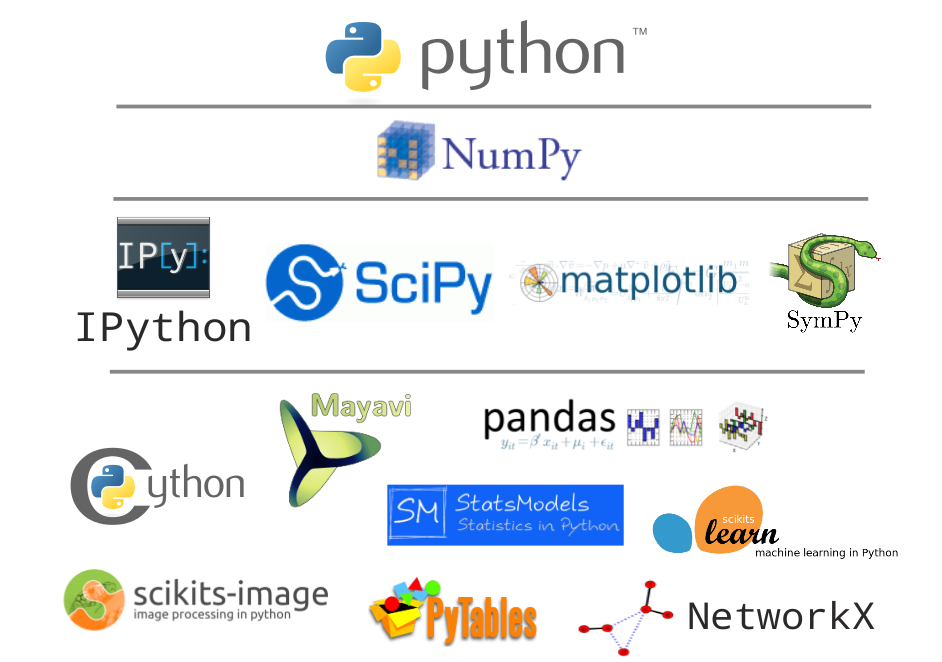
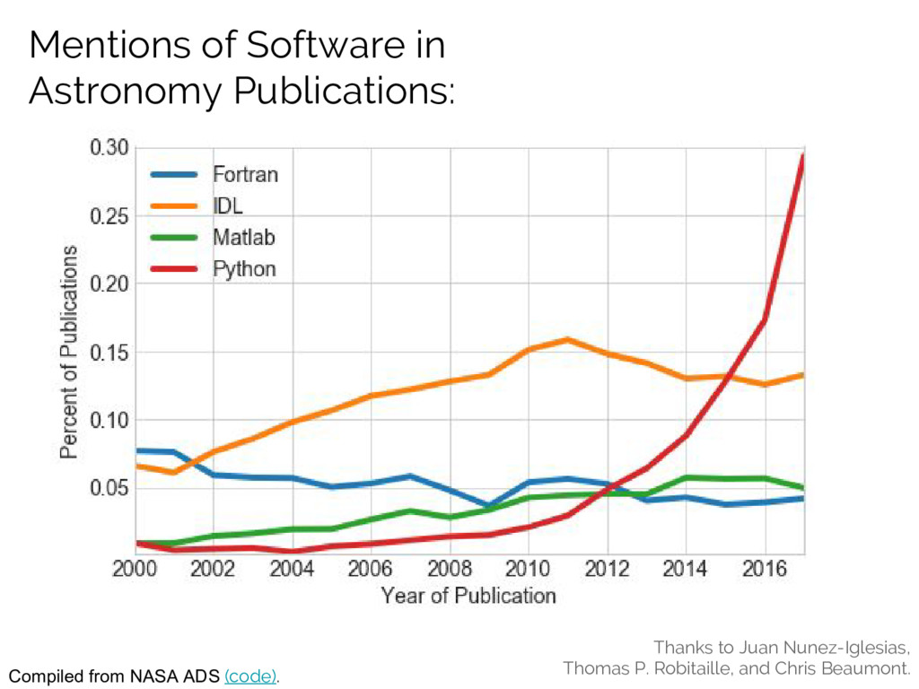
Why Python?
Pros
Versatile programming language with gentle learning curve
Easy to migrate. Very similar to MATLAB/Octave syntax
Interpreted, not compiled language
Automatic documentation, testing, code-coverage analysis
Cons
- Low performance compared to compiled languages C++, Fortran
Performance can be improved by offloading CPU intensive tasks to C++ or Fortran
INTRODUCTION
Why Python?
We should continue to move to higher levels of abstraction, just like we've done before. We should trade application speed for increased productivity, stability and maintainability. Programmer time is almost always more expensive than CPU time. We aren't writing applications in assembler anymore for the same reason we shouldn't be writing applications in C anymore. - From Haskell wiki
Example: Moving average filter algorithm - MATLAB vs Python
Note: without using any one-line functions
 v = .01; f = 100; fs = 5000; t = 0:1/fs:.03
 x = sin(2 * pi * f * t);                             %original signal
 r = sqrt(v) * randn(1, length(t));                %noise
 Xw = x + r;                                      %signal plus noise (filter input)
 y = zeros(___,'like',x)
 for n = 3:length(Xw),
    y(n) = sum(Xw(n - 2:n)) / 3;       %y[n] is the filtered signal
 end
 plot(y); hold; plot(x,'r');     %plot the original signal over filtered signal
 from pylab import *

 v = .01; f = 100; fs = 5000; t = arange(0, .03, 1 /fs)
 x = sin(2 * pi * f * t)                             # original signal
 r = sqrt(v) * random(len(t))                    # noise
 Xw = x + r                                      # signal plus noise (filter input)
 y = zeros_like(x)
 for n in range(3, len(Xw)):
    y[n] = sum(Xw[n - 2:n]) / 3       # y[n] is the filtered signal
 plot(y); plot(x,'r'); show()   # plot the original signal over filtered signal

FluidDyn project: a suite of Python packages for fluid dynamics
Open-source, documented, tested, continuous integration
- fluiddyn: base package containing utilities
- fluidlab: control of laboratory experiments
- fluidimage: scientific treatments of images (PIV)
- fluidfft: C++ / Python Fourier transform library (highly distributed, MPI, CPU/GPU, 2D and 3D)
- fluidsim: pseudo-spectral simulations in 2D and 3D
- fluidfoam: Python utilities for openfoam
Main developers: Pierre Augier (LEGI), Cyrille Bonamy (LEGI), Antoine Campagne (LEGI), Ashwin Vishnu (KTH), Julien Salort (ENS Lyon).

Numerical simulations
fluidsim: pseudo-spectral simulations in 2D and 3D
- solves Burgers, Navier Stokes, Shallow water, Föppl-von Kármán equations using a shared code base
- highly modular (object oriented solvers)
- efficient (Cython, Pythran, mpi4py, h5py)
- on-the-fly data processing
- built-in specialized plotting functions
fluidfft: unified API (C++ / Python) for FFT libraries (highly distributed, MPI, CPU and GPU, 2D and 3D)
%%capture
import fluidsim as fls

sim = fls.load_state_phys_file('/scratch/avmo/13KTH/toy_model_potential/SW1Lexmod_noise_c=12_Bu=1.0_L=50.x50._1920x1920_2017-05-13_05-03-26/')
%%capture --no-display
sim.output.spectra.plot2d(tmin=100, delta_t=0, coef_compensate=0.)

sim.output.phys_fields --no-display
sim.output.physkey_field=elds.plot(key_field='q')

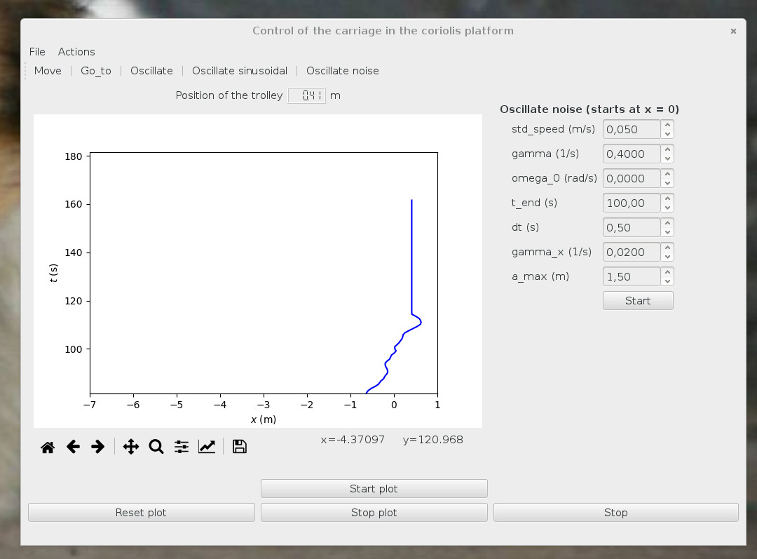
fluidlab: control of experiments in fluid mechanics
(Pierre Augier, LEGI & Julien Salors, ENS Lyon)
Physical experiments can be seen as the interaction of autonomous physical objects
- Object-oriented programming
- Very easy to write instrument drivers
- Automatic documentation for the instrument drivers
- Simple servers with the Python package
rcpy
Example for the carriage
motor.pyposition_sensor.pyposition_sensor_server.pyposition_sensor_client.pycarriage.pycarriage_server.pycarriage_client.py
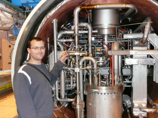
The MILESTONE experiment: stratified and rotating turbulence in the Coriolis platform
A collaboration between KTH, Stockholm, Sweden and LEGI, University of Grenoble, France
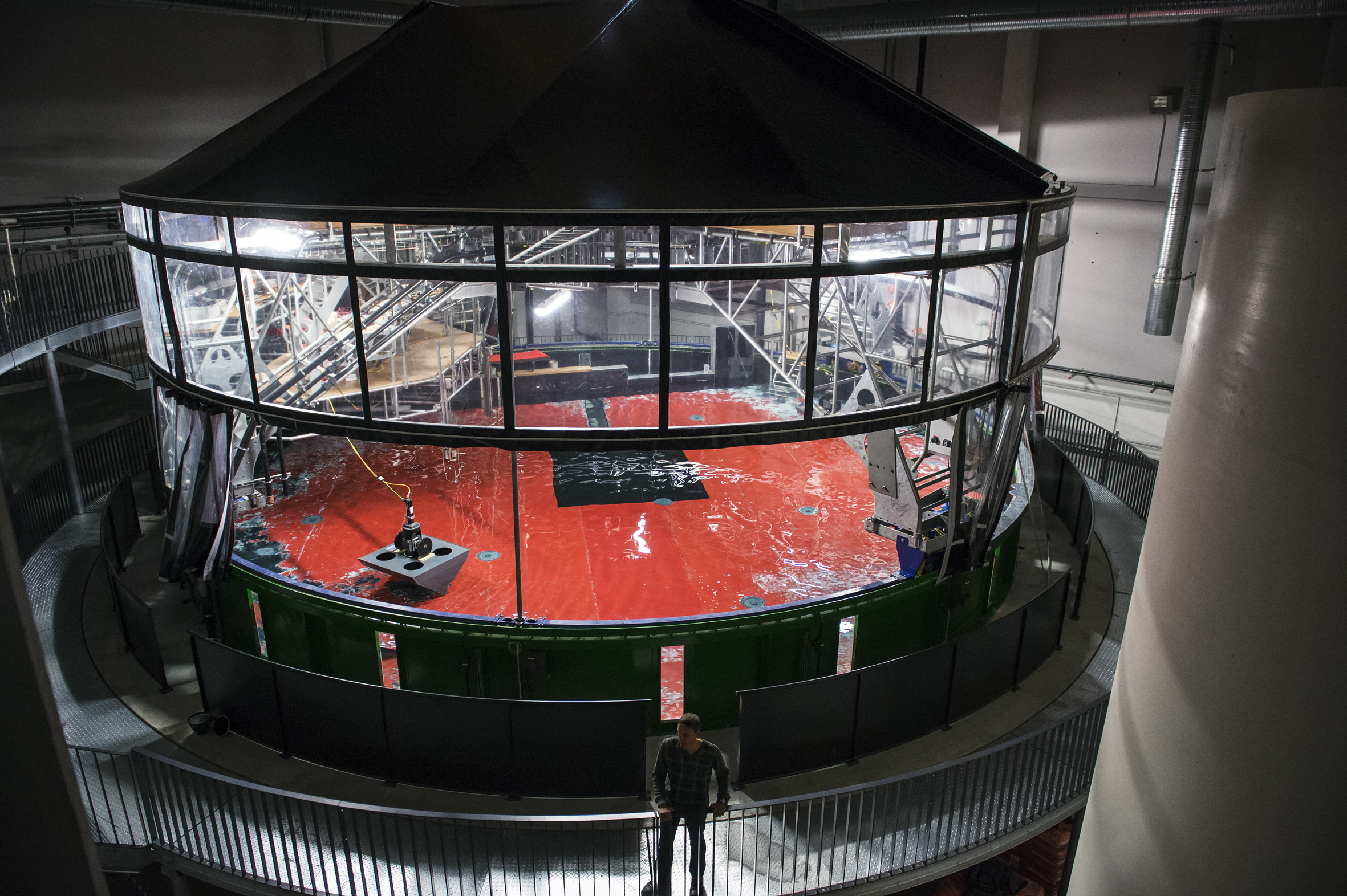
The Coriolis platform (13 m diameter)
Used by international researchers through European projects (Euhit, Hydralab).
fluidimage: scientific treatments of images
(Pierre Augier, Cyrille Bonamy & Antoine Campagne, LEGI; and Ashwin Vishnu, KTH)
Software for images preprocessing and Particle Image Velocimetry (PIV) computation
Many images (~ 20 To of raw data): embarrassingly parallel problem
- Clusters and PC
- CPU/GPU
- Asynchronous computations (topologies of treatments, IO and CPU bounded parts are splitted, compatible with big data frameworks as Storm)
- Efficient algorythms and tools for fast computation with Python (Pythran, Theano, Pycuda, ...)
2D and scanning stereo PIV
Utilities to display and analyze the PIV fields
- Plots of PIV fields (similar to PivMat, a Matlab library by F. Moisy)
- Calcul of spectra, anisotropic structure functions, characteristic turbulent length scales
fluidimage: PIV computation
Example of scripts to launch a PIV computation:
from fluidimage.topologies.piv import TopologyPIV

params = TopologyPIV.create_default_params()

params.series.path = '../../image_samples/Karman/Images'
params.series.ind_start = 1
params.piv0.shape_crop_im0 = 32
params.multipass.number = 2
params.multipass.use_tps = True
params.saving.how = 'complete'
params.saving.postfix = 'piv_complete'

topology = TopologyPIV(params, logging_level='info')
topology.compute()
Remark: parameters in an instance of fluiddyn.util.paramcontainer.ParamContainer. Much better than in text files or free Python variables!
- avoid typing errors
- the user can easily look at the available parameters and their default value
- documentation for the parameters (for example for the PIV topology)
fluidimage: Launching PIV computation on cluster
Remark: launching computations on cluster is highly simplified by using fluiddyn:
from fluiddyn.clusters.snic import Beskow

cluster = Beskow()

cluster.submit_script(
    'piv_complete.py', name_run='fluidimage',
    nb_nodes=1, nb_cores_per_node=8, email='johndoe@kth.se')
Partial conclusion: Open-data, data in auto-descriptive formats (hdf5, netcdf, ...) + code to use and understand the data.
Conclusions
Science in fluid mechanics with open-source methods and Python
Development of open-source, clean, reusable codes (fluiddyn project)
Issues
- Collaborative dynamics? Adoption by scientists? Developers?
- Level in Python and coding in the community ! => Python training sessions in the lab and at university